ArcGIS Spatial Statistics and Network Analysis
28 Mar 2013 - by @黄野1. Background study
According to the Finnish law, the municipalities are obliged to offer day care to all children under school age. The school is usually started in the autumn of the year when the child is 7 years old. Although the right for day care is universal, the practical situation varies. Usually babies and very young children stay at home, but the age when the parents return to work and put the child in day care varies considerably. The municipalities also cooperate with neighbouring municipalities and private kindergartens in arranging the day care. Nevertheless, the most usual way for municipalities is to allocate the children in municipally operated day care centres.
Arranging the day care in municipalities and areas with rapid growth of families is always a difficult task. According to the Finnish newspaper HelsinginSanomat (21.11.2012), in many areas of the city of Helsinki there are more children than day care places. The parents may have several preferences in choosing the day care centre, but the proximity to home is most likely a key factor to the majority. At least in Helsinki the closest preschool is usually the preferred one (HelsinginSanomat 3.12.2012).
2. Scenario: Day-care centers planning in Espoo, Finland
In our project work we are concentrating on the municipal day care centres in the city of Espoo. Espoo is the second biggest municipality in Finland and its population is growing over 1% yearly, mainly from birth rate (City of Espoo 2012). It’s plausible that the network of municipal day care centres has difficulties in keeping up with the growing child population. In our scenario we are going to analyse patterns of children and municipal day care centres for the use of Espoo day care administration.
For practical purposes we are making some assumptions to limit our research efforts. Firstly, we are taking into account only the municipal day care centres. In practice the city of Espoo needs cooperation both with neighbouring municipalities and private kindergartens. Our analysis can spot the areas where these kinds of arrangements are most likely needed. Secondly, we assume the parents to prioritize the option closest to their home. Although this is not far from truth we are forced to make this assumption as there is no data from real choices or preferences. Finally, we assume that all children from 1 to 7 years old would apply for municipal day care. In real world many of the younger children would stay at home. But once again we lack the data to model the share of children staying at home. Our analysis also shows the potential maximum stress directed to the day care system. As the planning, decision-making and implementing takes time, we analyse the children from 0 to 6 years old, assuming them to be one year older when the planning process is over.
3. Useful cases and data
Our research is divided into three use cases:
- Spatial distribution of children population
- Spatial distribution of day care centres and their buffer areas to understand if they are sufficient or not for the closest population
- The closest centres according to the driving speed and walking distance
We are using data from three sources:
- The address, size and occupancy of day care centres were obtained from the city of Espoo in Excel form. The day care centre data had to be cleaned and combined before geocoding it in ArcGIS.
- The data of child population was taken from SeutuCD 2008, where the population in different age groups by the residential building were stored in a database file.
- For the accessibility analysis we used Digiroad data obtained from Paituli service.
One notable problem with the data is the gap in time perspective. We were able to use current day care centre data, but the most recent population data available for our project work is from 2008. The four year gap leads to some odd results in the analysis that must be taken into account when making conclusions.
4. Children distribution in Espoo
Initial data: SETU Vaki - Children from 0 to 6 years old who live in all houses in Espoo. 29115 addresses and 22850 children in total.
The goal of analysis: To find some patterns of children distribution in Espoo – clustering, density or if spatial autocorrelation in their distribution exists.
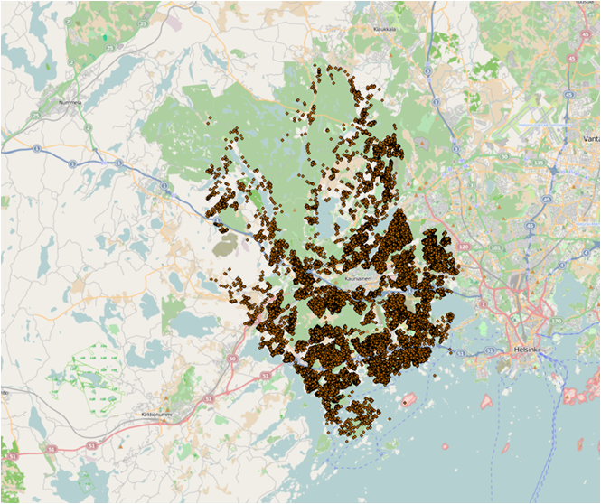
Figure 1 Children distribution in Espoo
4.1. Analysis of children distribution in Espoo
(1)Kernel Density: Demonstrates the spatial distribution of phenomena using function summing overlapping values of frequency in each point of area.
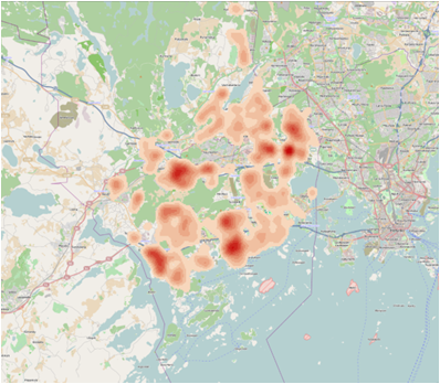
Figure 2 Kernel Density of the children distribution in Espoo. Output cell – 76,3 (default), Search radius – 636 (default) sq km
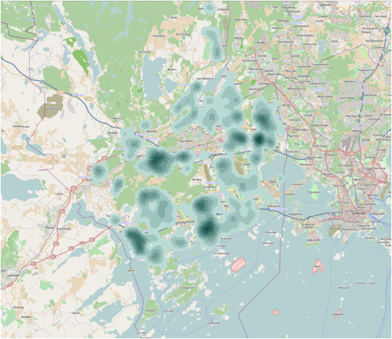
Figure 3 Output cell – 100, Search radius – 636 (default) sq km
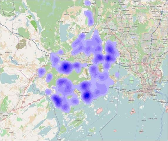
Figure 4 Output cell – 100, Search radius – 800 sq km
Result: Visualization if children density allowed us to define several parts of Espoo with very high density of children population:
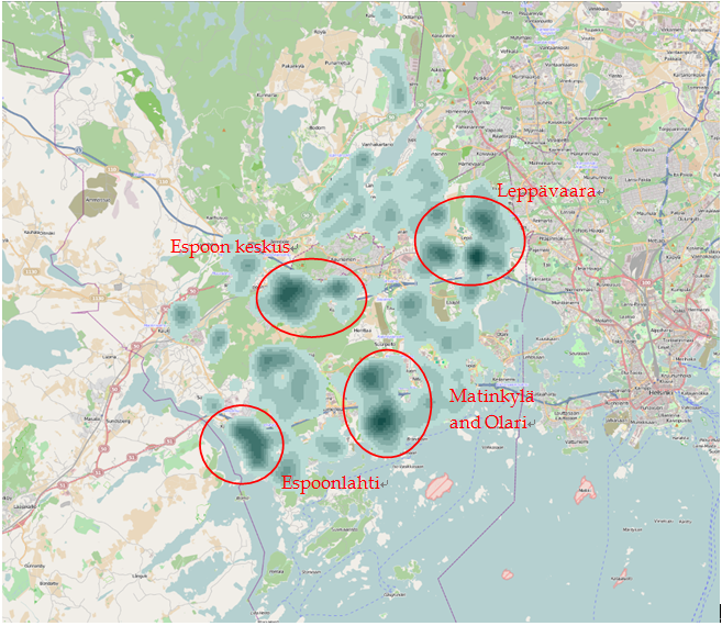
Figure 5 Several parts of Espoo with very high density of children population
(2)Nearest Neighbor Clustering : Method allows to find clusters in the pattern of phenomena distribution.
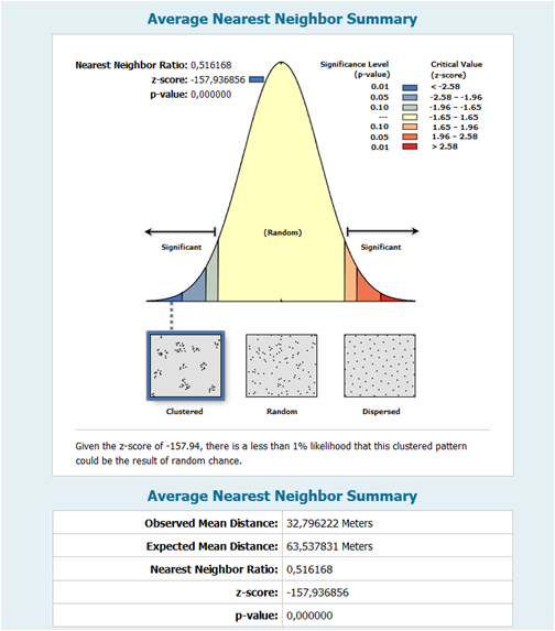
Figure 6 The summary of average nearest neighbor shows the distribution of children population is significantly clustered, which statistically approves our initial hypothesis about the clustering of children distribution
(3)Spatial Autocorrelation (Global Moran’s I) : Tool measures spatial autocorrelation based on both feature locations and feature values simultaneously. Given a set of features and an associated attribute, it evaluates whether the pattern expressed is clustered, dispersed, or random.
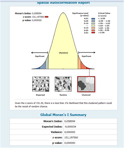
Figure 7 The report of spatial autocorrelation shows that our point pattern is significantly clustered (p-value « 0.01 and z-score » 2.58). It means that we may reject our null hypothesis. The children population spatial distribution of high values and/or low values (The number of children in each building) in the dataset is more spatially clustered than would be expected if underlying spatial processes were random
(4)Hot Spot Analysis (Getis-Ord Gi) : Given a set of weighted features, identifies statistically significant hot spots and cold spots using the Getis-Ord Gi* statistic
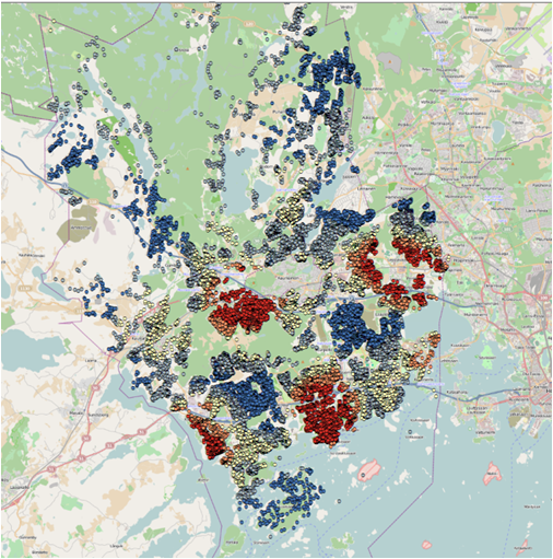
Figure 8 The region of red color represents the statistically significant spatial clusters of high children population density while the blue color identifies the significant spatial clusters of low children population density
Result: Red dots are clusters with high values, blue are with lowest values. We found that in some places in Espoo the concentration of children is very high what might be connected this higher housing density. To approve this hypothesis we applied Kernel density for housing data.
4.2. Analysis of houses distribution in Espoo
(1)Kernel Density of houses distribution
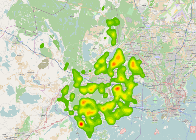
Figure 9 Kernel Density of houses distribution
Result : Visualization of housing density approved our hypothesis and we can definitely say that children distribution has the same pattern, as the entire population and depends only from housing factor. There were revealed no abnormal facts that would lead to a deviation from the normal distribution.
5. Day-care centers distribution in Espoo
Initial data: Day-care centers data from the institution of Espoo day care planning, containing both the number of day care places in each centre and the number of children currently in those facilities. Three main attributes for the day care centres are collected: locations - (X,Y) coordinates and text addresses, day care centers total - 136 day care centers, day care centers occupied: (a)The theoretical or planned size of the centre (represented by the field ‘Places’), (b)The real number of children currently exist in the centers (represented by the field ‘Kids’), (c)The difference between the theoretical size and the real size of day-care centers (represented by the field ‘Difference’, and if ‘Difference’ is positive, the centre could easily take in more kids, otherwise, the centre is already overcrowded, at least according to the initial plans).
The goal of analysis: Analyze the distribution(clustered or dispersed) of day-care centres and the distribution of children in those day-care centers by using the spatial statistics tools. And because of the limitation of data, we just evaluate two kinds of value in each analysis. One is regarded the number of children in every day-care center as the input value, the aim is to find some abnormal values of the children distribution based on the day-care-center-unit(for example, the number of children in one care center is obviously more than the number of children in other care centers which are around it). The other is regarded the number of day-care center as the input values, the aim is to find some abnormal values of the care centers distribution(for example, find the cluster regions of day-care center).
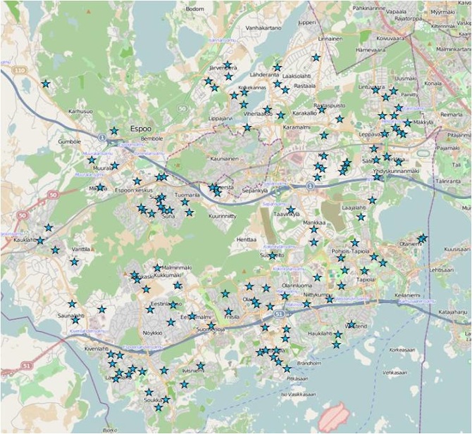
Figure 10 The distribution of Day-care centers in Espoo
5.1 Analysis of Day-care centers distribution in Espoo
(1) Kernel Density
Basic research idea: the syntax of Kernel Density in ArcGIS is
Kernel Density(in_features, population_field, {cell_size}, {search_radius},{area_unit_scale_factor}). The last 3 items are optional. In terms of care centers, the parameter in_features is the point feature class of care centers and the parameter population_field shold be set as NULL so that the volume under the surface equals the Population field value for the point (here is 1, and means each point represents just one care center).However, in terms of children’s population, as the number of children in each location aggregate in building level(each point reprents a building and there must be a field in the attributes table showing the chirdren’s total population of each building), we need to set the parameter population_field as the number of children in each building so that times that each point will be counted are the number of children in this point.
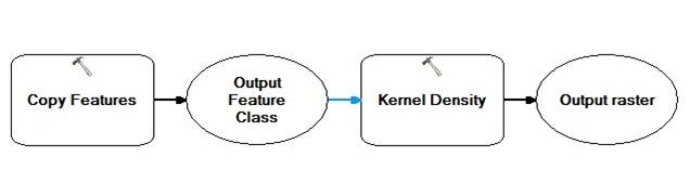
Figure 11 The workflow of kernel density of the day-care centers
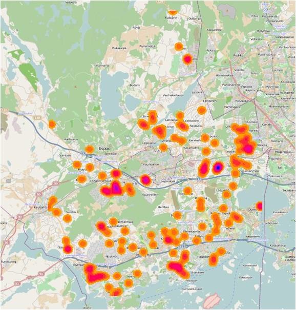
Figure 12 The outcome of the analysis. Blue parts show that the number of day-care centers in those regions present peaks
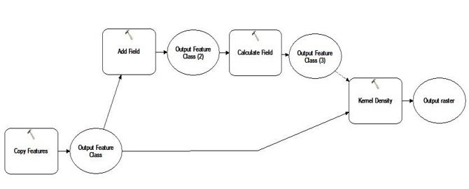
Figure 13 The workflow of kernel density of children distribution in day-care centers. The steps of “Add field” and “Calculate field” are used to define the “Population” field in ArcGIS as the total number of children in each day-care center
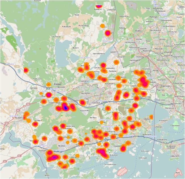
Figure 14 Blue parts show that the number of children in those day-care centers present peaks
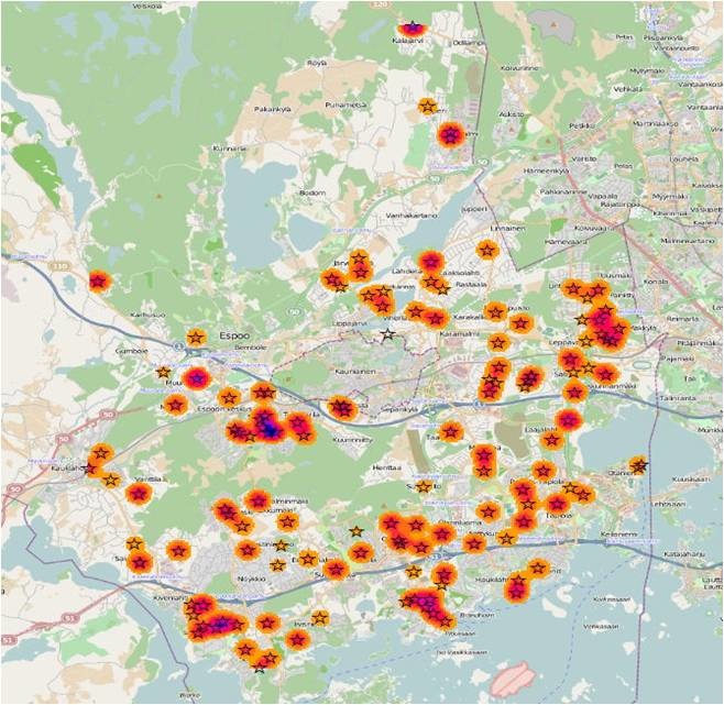
Figure 15 Combined with the distribution of care centers, we can find that some of the cluster areas of care centers are not the cluster regions of children
(2) High/Low Clustering(Getis-Ord General G)
Basic research idea: firstly, we are going to integrate care centers by specifying range constraint (The “Integrate Tool” provides this function) and then use the “Collect Events Tool” to calculate how many care centers in each point so that differences of the number of day-care centers between those points on the map can be defined as the high/low value. Finally, I will apply the High/Low Clustering to analyze the spatial distribution of those points by using Getis-Ord General G method.
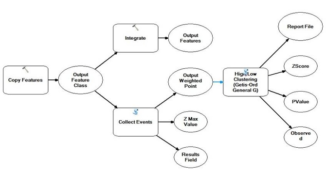
Figure 16 The workflow of High/Low Clustering of day-care centers distribution
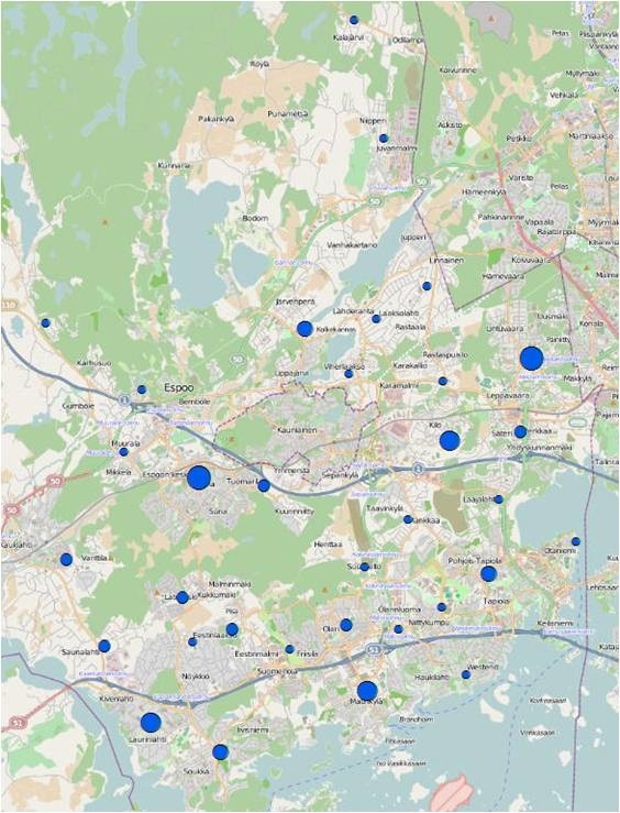
Figure 17 The outcome of steps of “Integrate” and “Collect events”. The X,Y tolerance is 500 meters. Bigger circles mean more day-care centers are integrated in those regions, while smaller circles mean less day-care centers are located in those regions. It’s easy to observe that the high-value point repels other high-value points while the low-value points also present a situation of random distribution
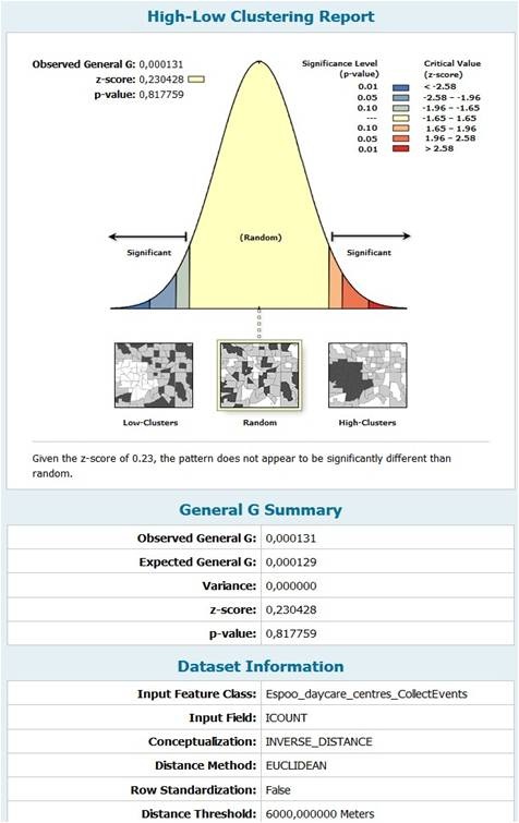
Figure 18 The report shows that the high value or the low value of the number of care centers are randomly distributed, which means the observed spatial pattern could very well be one of many possible versions of complete spatial randomness (CSR). Therefore, I cannot find any potential information, such as “some day-care centers are more competitive because of their better teaching facilities or high quality of teachers” or “some day-care centers are more popular because the population there is more dense”, through this analysis
(3) Hot Spot Analysis
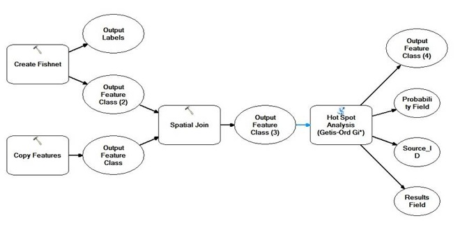
Figure 19 The workflow of Hot Spot Analysis of children pattern which uses the “fishnet” and “sptial join” to integrate the number of chilren in day-care centers falling within each grid polygon
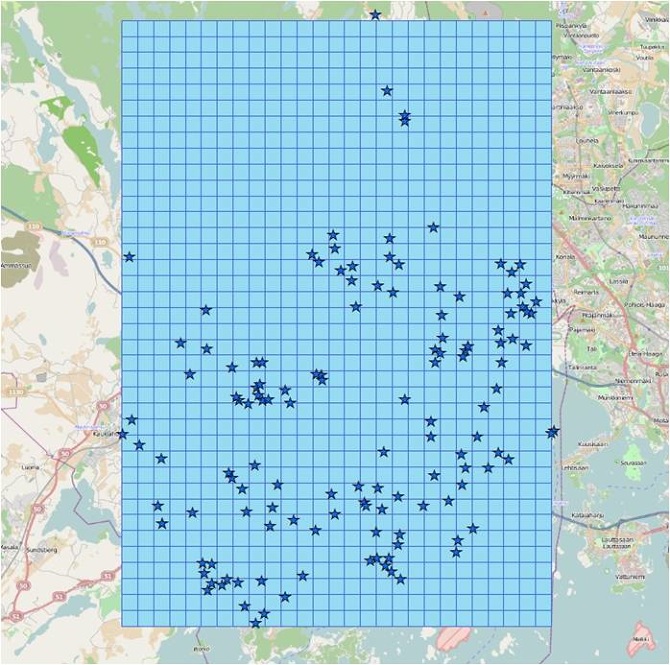
Figure 20 The “fishnet” is created as the traget feature class of the “spatial join”
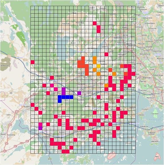
Figure 21 The final result of Hot Spot Analysis, some significantly clustered region of high value (blue part) and low value (yellow part) can be explicitly identified
PS: It makes sense that the blue part is located in that specific place because lots of day-care centers and more children are gathered there. However, I do find a abnormal value (a purple grid) which exists right at the lower-left side. Actually, there is only one day-care center falling in that grid, but why it shows a sort of high-value trend? Therefore, I think my next plan is tring to dig out the background information of that day-care center, and maybe I can find the reason why this day-care center is so popular.
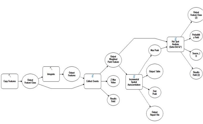
Figure 22 The workflow of Hot Spot Analysis of care centers pattern
PS: The outcome of Incremental spatial autocorrelation shows no valid peaks found at the specified distances because of the significant peak z-scores are not found. So here I tried to use 4000 meters (default), 8000 meters and 10000 meters as the distance thresolds of fixed_distance_band. Due to we have no enough data, here the conceptualization of spatial relationships which is set as “fixed_distance_band” is proper. Because the parents will not choice far day-care centers for their children, those centers out of a fixed distance will not influence each other. However, if we have enough data, each kind of data is regarded as a factor that will influence the decision-making of the parents, maybe it will lead to the change of conceptualization of spatial relationships.
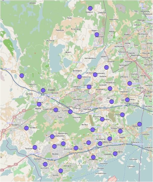
Figure 23 The distance band was set as 4000 meters. No abnormal values was found
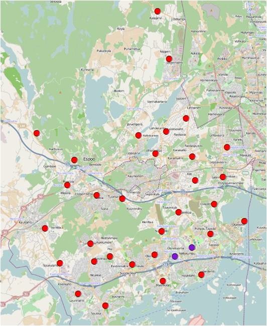
Figure 24 The distance band was set as 8000 meters, and 2 significant spatial clusters of high value were identified
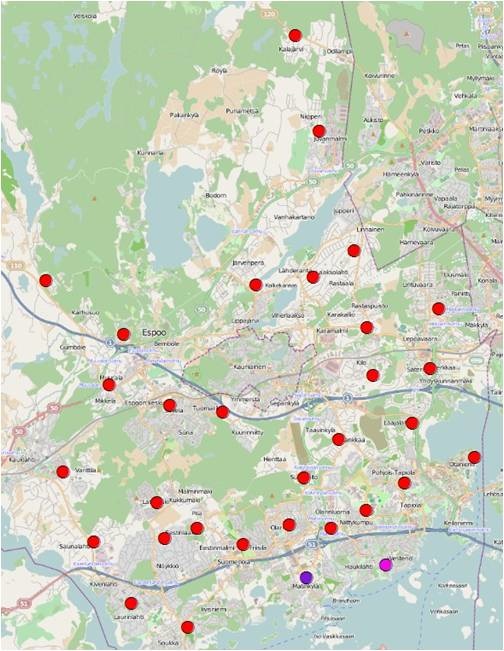
Figure 25 the distance band was set as 10000 meters, and another 2 significant spatial clusters of high value were identified.
PS: If we change the distance band to a proper distance, more elements will be took into account so that we can find out some abnormal value in parts.
6. The closest day care centre by driving and walking
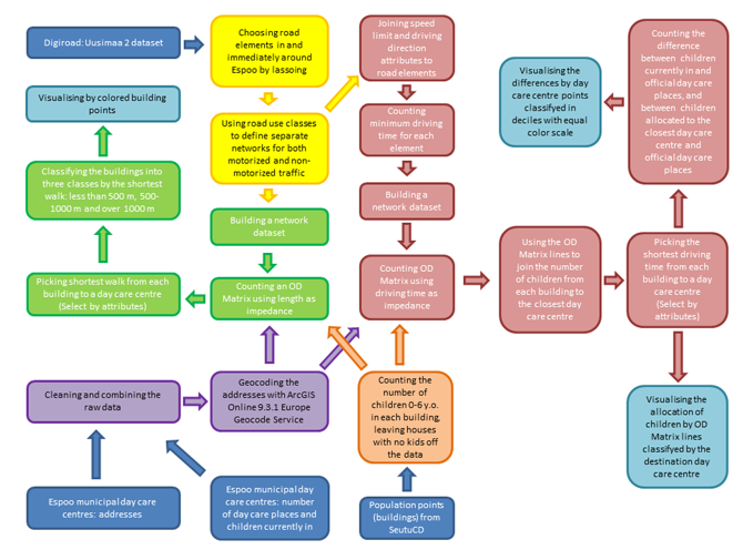
For the third use case we used network analysis to define the closest day care centre and the minimum walking distances. The network (or networks, as we had to take into account the vehicle restriction in different roads) was built using the Digiroad data obtained from PaITuli service. The initial data covered large parts of the Uusimaa region, so the study area had to be minimized, because the dataset is huge and heavy to calculate. The road use classes were ready in the LIIKENNE_ELEMENTTI file, but the speed limit and driving direction attributes had to be joined by reference codes from the LIIKENNE_SEGMENTTI file. In building the networks both the length and the minimum driving time calculated with the speed limit (assumed 50 km/h if no data) were used as the impedance. Road classification was used as the hierarchy and the dummy variables formed from the driving direction variable were linked to the corresponding direction to deny the possibility to drive against the flow. Initially the Closest Facility algorithm was tried but the size of the data forced us to use the OD Matrix algorithm instead. The diagram of the complete work flow is presented below.
(1) The closest facility (Day-care centers)
Basic research idea : we can calculate the driving times from the residential buildings to the day care centres. The closest options with the shortest driving time are selected from the complete matrix and the allocation of the houses with child population to the closest day care centres is visualized below.
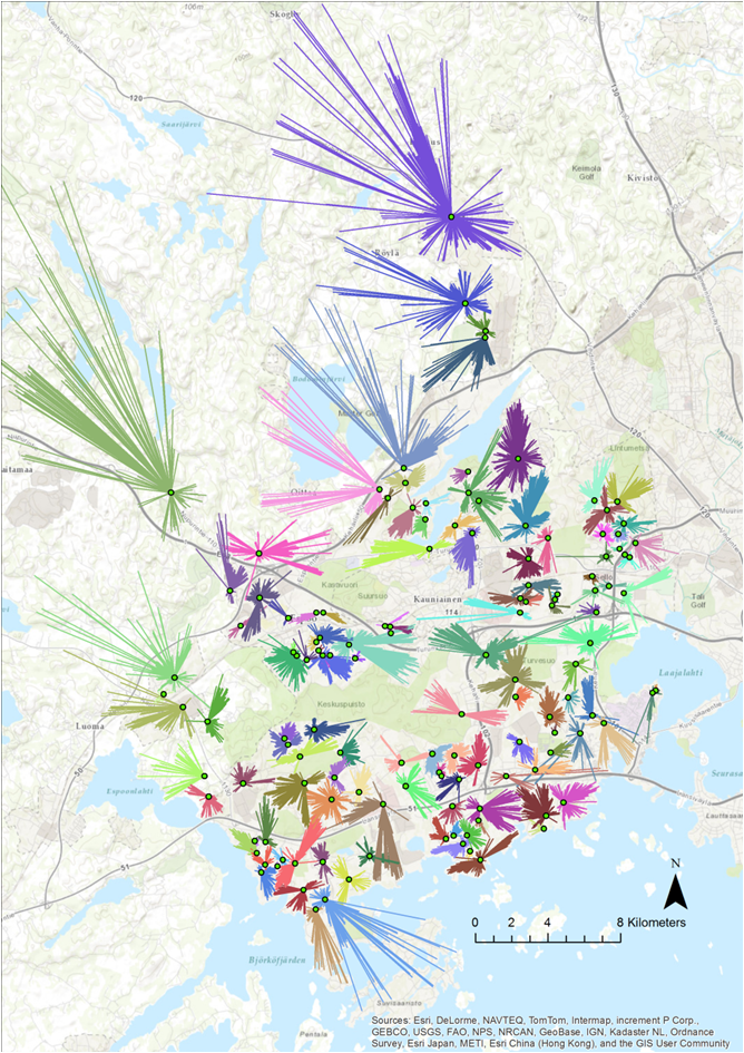
Figure 27 The closest day care centre by the driving time
PS: Overall the driving times were short, although the estimation is not fully realistic as rush hour traffic hardly follows the maximum speed limit. Notably the clustered nature of day care centres in the densely built areas mean that the closest option is practically at the same distance as the second or third closest ones. The optimal service area is clearer in the northern outskirts of Espoo, where the distances and travel time can be longer, too.
(2) The actual crowdedness and potential stress to day-care centres
Basic research idea : the allocation of buildings to the closest day care centre was used to model the potential stress directed to the existing day care centre network. The number of 0-6 year old child population from the buildings were first joined by location to the OD Matrix lines and subsequently summed to the day care centres in the other end of the line. The number of children, whose closest option the day care centre was, was compared to the official size of the centre. The same comparison was made to the actual current number of children and the official size. The differences were categorized into deciles and visualized with the same colour scale.
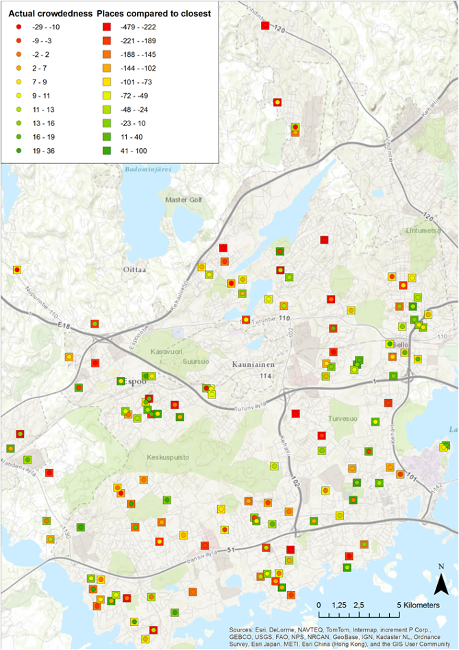
Figure 28 The actual crowdedness and the potential stress to day-care centres
PS: It is very clear that the municipal day care cannot cope without the help of home parents and other day care facilities. The dense areas are generally well served. The clustering nature of day care centres means that in many areas our rigid analysis of closest options results high and low stress centres being next to each other. In some areas the actual and potential crowdedness correspond. In these areas the day care network seems to have gaps. Those areas tend to be in the northern part of the area or between major suburbs but with high accessibility by the road network.
(3) Walking distance to the closest day-care centre
Basic research idea : we built a different network for non-motorized traffic and analysed the walking distances. The shortest distances obtained from the OD Matrix tool were classified in three bands: less than 500 m, 500-1000 m, and over 1 km. The buildings were color-coded by the classification and the resulting map is shown in the figure 29 below.
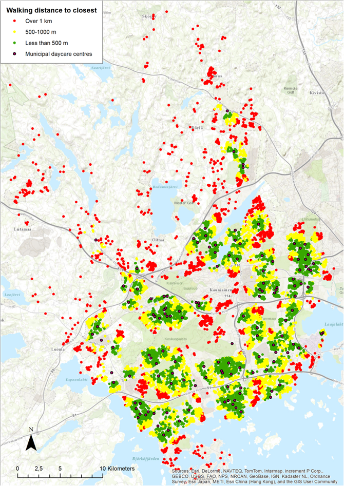
Figure 29 Walking distance to the closest day care centre
PS : It is no surprise that in the outskirts of Espoo the day care centres are mainly off the walking distance. The sparse network of single-family houses makes the maintenance of close-by day care centres economically unviable. More could be done in the edges of bigger suburbs, where the day care centres tend to be located in the central areas, leaving many houses over 1000 metres away from the closest facility. Interestingly there is one seemingly misplaced centre in the Central Espoo: according to figure 28 it is relatively empty but there are large areas with long distances just nearby. One reason to the oddity is the time gap in the data: the day care centre data is recent, but population data from 2008. In real life the area is under major development with new houses already built after 2008. Overall in our analysis 50% of the children (44% of the houses) have a municipal day care centre less than 500 metres away, and 16% of the children (20% of the buildings) would have to walk more than 1 km.
7. Conclusion
Our analysis shows that the child population is heavily concentrated to the generally densely built suburbs. The result is obvious both from visual and statistical analysis. Those suburbs are also well served with municipal day care centres. Families have usually short walk to a centre and there are many options practically next to each other.
Still, some of the day care centres are not co-located with the children. Either concentrations of child population lack a day care centre nearby, or the centre seems to be in the middle of unbuilt area. Especially in the latter case the time gap in the data hides the fact that some areas are under development and already in need of municipal services.
It is not a surprise that the northern areas of Espoo suffer from long travel times, lack of walking distance options and already crowded day care centres. The latter fact proves the difficulties of municipal services to adapt to rapidly growing population. Some new developments are definitely needed in those areas but in general the low density makes the building of service network economically hard.
Another clear fact by far is the total amount of children is a bit overloaded for those day care centres in the municipal and the day care system simply could not be able to take in all the small children currently. Therefore, some cooperations with private kindergartens and other municipalities become more important.
Team work by Ye Huang, Anna Gorodetskaya and Simo Syrman